The first item to understand is that from day one, every oil and gas well is a declining asset. Typically, there is a fixed amount of oil and gas that the well will provide over its lifetime and each day the well produces, the remaining uncoverable amount decreases. Petroleum engineers pay close attention to this phenomenon, using what the industry calls a decline curve.
This article discusses the technical aspects of a decline curve. The curve illustrates the production rate of a well through its life span. By the end of the article you will understand the 3 types of decline curves, how they are applied, and why they are important throughout the industry.
What are Decline Curves?
Decline curves are one of the oldest methods used for predicting the future of oil and gas well production. In theory, they apply to most wells in the industry. Once an oil and gas well has been completed (the process of making a well ready for production), its maximum production level can be attained within days or weeks. After this level has been reached (transient flow period), there is a decline in production usually caused by loss of reservoir pressure or changing volumes of produced fluid. The rate of production decline is depicted by a decline curve. Decline curves generally show the amount of oil or gas produced per unit of time, for many successive periods.
Decline curves are generated from Decline Curve Analysis (DCA) software. They utilize past production history of a petroleum reservoir to create a well production profile. Production decline curves assist in determining well performance, life expectancy, present and future production, and also profitability of a field.
How Decline Curves Are Applied
DCA is used to help predict the future production of wells, and determine future cash flow. This information can be used to determine the value of the mineral rights or land. The analysis of well depletion and discounted future cash flow is imperative information for oil and gas operators. It is especially important when estimating the cost of buying or leasing mineral rights, paying royalty owners, and understanding the economic impacts of acquiring other assets.
The 3 Types of Decline Models
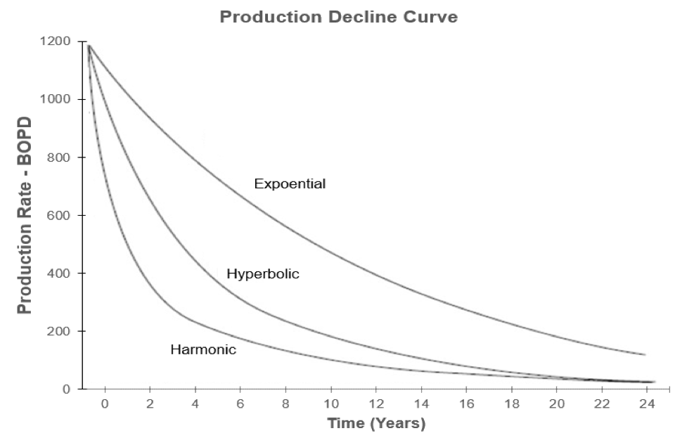
Typically, DCA involves examination of three types of basic production decline models. The models are Exponential, Hyperbolic and Harmonic (Figure 1). These models were first developed by J.J. Arps. The models show trend lines that best fit the production profile of a well, indicated by the production rate (y-axis) over a continuous time period (x-axis).
Technical Details of the 3 Decline Models
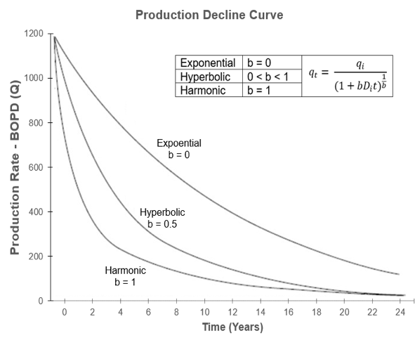
Figure 2 shows a graphical representation of the 3 types of models. In the equation below, qi= initial production rate, qt= the production rate at the given time, t= time, Di=initial decline fraction, b= hyperbolic exponent from (0 to 1). The equation shows that the respective decline curves are generated based on the value of b. The b factor regulates the initial steepness of the decline curve.
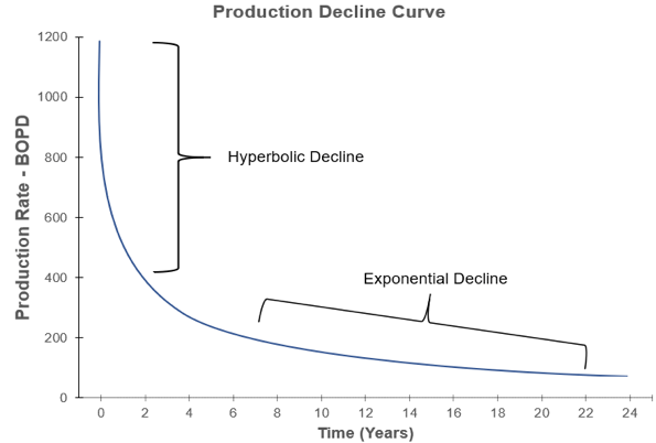
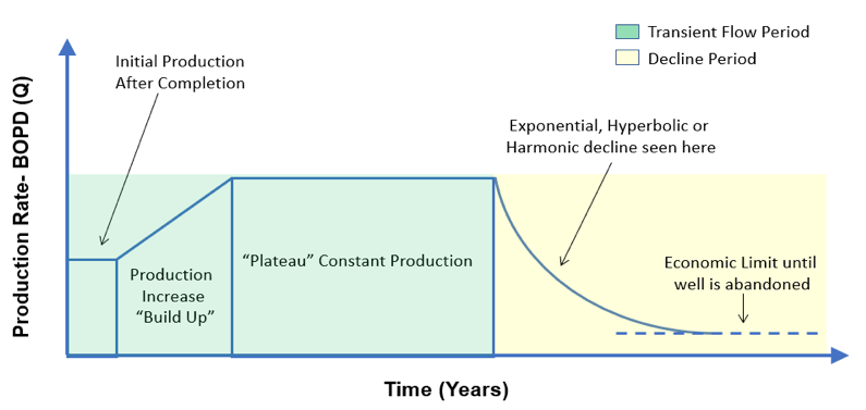
Although a decline curve can be depicted by one of the models shown above, in many cases the decline is represented by an assimilation of the hyperbolic and exponential models. It has been seen that hyperbolic or harmonic models have historically tended to overestimate cumulative production. Due to this, a conservative model will normally have a “transition” point in which a hyperbolic or harmonic decline will transition to an exponential decline. For example, Figure 3 shows a well that may initially have a steep drop in production denoted by the hyperbolic decline. It then transitions to a more constant and steady decrease in production denoted by the exponential decline.
It is important to note, that the decline curve models are only applicable after the transient flow period of a well. The transient flow period is the initial production experienced by a new oil & gas well, when no reservoir boundaries have been reached. During this period, a well normally has constant and steady pressure from the reservoir. The decline curves are applicable after the “plateau” (See Figure 4). In many shale fields, the transient flow period may be very short, and production decline begins almost immediately. Figure 3 depicts the life cycle of an oil & gas well.
Why Decline Curves Matter to Mineral Rights Holders and Royalty Owners
The 3 decline curves mentioned above are important because they are used as one of the factors in determining the value of minerals or land. Oil & gas companies normally gather data on existing wells which exhibit similar characteristics (Reservoir formation, depth of well, reservoir pressure, etc.) to the new well they intend to drill. The decline curve that most closely fits the nature of the new well is used, and extrapolated to create a predicted model for the new well. From this decline curve, a cumulative production rate can be estimated over a specific time frame. Ultimately a future cash flow is determined, and a net present value (NPV) can be calculated. This NPV is what gives value to the mineral rights, and land that oil and gas companies are trying to buy or lease.
Where You May Encounter Decline Curves?
The invaluable information from production decline curves is commonly used for economic forecasting, financial modeling, investor presentations, lease analysis and property valuation. This is due to the direct correlation of well production rates to present and future cash flow of an oil & gas field. The data can be used to determine the financial strength or weakness of a company’s present and future activities, by evaluating potential return on revenue (ROR). Many operating companies use the data when accounting for depreciation charges in their books as well.
In addition to the use of decline curves on the economic/financial side, they are also used for technical analysis. Completions engineers use the models to evaluate the outcomes of new completion techniques in a specific area. Production engineers use the models for planning enhanced recovery methods (Water flood, CO2 injection, produced gas injection, etc.) to sustain or increase well production levels.
Summary
As described above, decline curve models are a very important tool in the oil and gas industry. They are especially useful for operators, mineral rights owners, royalty owners, and production/completions engineers. By using proper DCA techniques, the models provide valuable forecasting for well performance, life expectancy and cash flow. This information is critical for mineral rights owners trying to buy or sell mineral rights at a fair price, and also royalty owners looking for proper payment on their oil and gas interests.